Run Cumulus for sc/snRNA-Seq data analysis
Run Cumulus analysis
Prepare Input Data
Case One: Sample Sheet
Follow the steps below to run cumulus on Terra.
Create a sample sheet, count_matrix.csv, which describes the metadata for each sample count matrix. The sample sheet should at least contain 2 columns — Sample and Location. Sample refers to sample names and Location refers to the location of the channel-specific count matrix in either of
10x format with v2 chemistry. For example,
gs://fc-e0000000-0000-0000-0000-000000000000/my_dir/sample_1/raw_gene_bc_matrices_h5.h5.10x format with v3 chemistry. For example,
gs://fc-e0000000-0000-0000-0000-000000000000/my_dir/sample_1/raw_feature_bc_matrices.h5.Drop-seq format. For example,
gs://fc-e0000000-0000-0000-0000-000000000000/my_dir/sample_2/sample_2.umi.dge.txt.gz.Matrix Market format (mtx). If the input is mtx format, location should point to a mtx file with a file suffix of either ‘.mtx’ or ‘.mtx.gz’. In addition, the associated barcode and gene tsv/txt files should be located in the same folder as the mtx file. For example, if we generate mtx file using BUStools, we set Location to
gs://fc-e0000000-0000-0000-0000-000000000000/my_dir/mm10/cells_x_genes.mtx. We expect to seecells_x_genes.barcodes.txtandcellx_x_genes.genes.txtunder foldergs://fc-e0000000-0000-0000-0000-000000000000/my_dir/mm10/. We support loading mtx files in HCA DCP, 10x Genomics V2/V3, SCUMI, dropEST and BUStools format. Users can also set Location to a foldergs://fc-e0000000-0000-0000-0000-000000000000/my_dir/hg19_and_mm10/. This folder must be generated by Cell Ranger for multi-species samples and we expect one subfolder per species (e.g. ‘hg19’) and each subfolder should contain mtx file, barcode file, gene name file as generated by Cell Ranger.csv format. If it is HCA DCP csv format, we expect the expression file has the name of
expression.csv. In addition, we expect thatcells.csvandgenes.csvfiles are located under the same folder as theexpression.csv. For example,gs://fc-e0000000-0000-0000-0000-000000000000/my_dir/sample_3/.tsv or loom format.
An optional Reference column can be used to select samples generated from a same reference (e.g. mm10). If the count matrix is in either DGE, mtx, csv, tsv, or loom format, the value in this column will be used as the reference since the count matrix file does not contain reference name information. The only exception is mtx format. If users do not provide a Reference column, we will use the basename of the folder containing the mtx file as its reference. In addition, the Reference column can be used to aggregate count matrices generated from different genome versions or gene annotations together under a unified reference. For example, if we have one matrix generated from mm9 and the other one generated from mm10, we can write mm9_10 for these two matrices in their Reference column. Pegasus will change their references to mm9_10 and use the union of gene symbols from the two matrices as the gene symbols of the aggregated matrix. For HDF5 files (e.g. 10x v2/v3), the reference name contained in the file does not need to match the value in this column. In fact, we use this column to rename references in HDF5 files. For example, if we have two HDF files, one generated from mm9 and the other generated from mm10. We can set these two files’ Reference column value to mm9_10, which will rename their reference names into mm9_10 and the aggregated matrix will contain all genes from either mm9 or mm10. This renaming feature does not work if one HDF5 file contain multiple references (e.g. mm10 and GRCh38).
The sample sheet can optionally contain two columns - nUMI and nGene. These two columns define minimum number of UMIs and genes for cell selection for each sample in the sample sheet. nGene column overwrites minimum_number_of_genes parameter.
You are free to add any other columns and these columns will be used in selecting channels for futher analysis. In the example below, we have Source, which refers to the tissue of origin, Platform, which refers to the sequencing platform, Donor, which refers to the donor ID, and Reference, which refers to the reference genome.
Example:
Sample,Source,Platform,Donor,Reference,Location
sample_1,bone_marrow,NextSeq,1,GRCh38,gs://fc-e0000000-0000-0000-0000-000000000000/my_dir/sample_1/raw_gene_bc_matrices_h5.h5
sample_2,bone_marrow,NextSeq,2,GRCh38,gs://fc-e0000000-0000-0000-0000-000000000000/my_dir/sample_2/raw_gene_bc_matrices_h5.h5
sample_3,pbmc,NextSeq,1,GRCh38,gs://fc-e0000000-0000-0000-0000-000000000000/my_dir/sample_3/raw_feature_bc_matrices.h5
sample_4,pbmc,NextSeq,2,GRCh38,gs://fc-e0000000-0000-0000-0000-000000000000/my_dir/sample_4/raw_feature_bc_matrices.h5
If you ran cellranger_workflow previously, you should already have a template count_matrix.csv file that you can modify from generate_count_config’s outputs.
Upload your sample sheet to the workspace.
Example:
gsutil cp /foo/bar/projects/my_count_matrix.csv gs://fc-e0000000-0000-0000-0000-000000000000/
where
/foo/bar/projects/my_count_matrix.csvis the path to your sample sheet in local machine, andgs://fc-e0000000-0000-0000-0000-000000000000/is the location on Google bucket to hold it.Import cumulus workflow to your workspace.
Import by following instructions in Import workflows to Terra. You should choose github.com/lilab-bcb/cumulus/Cumulus for import.
Moreover, in the workflow page, click the
Export to Workspace...button, and select the workspace to which you want to export cumulus workflow in the drop-down menu.In your workspace, open
cumulusinWORKFLOWStab. SelectRun workflow with inputs defined by file pathsas below
and click the
SAVEbutton.
Case Two: Single File
Alternatively, if you only have one single count matrix for analysis, you can go without sample sheets. Cumulus currently supports the following formats:
10x genomics v2/v3 format (hdf5);
Drop-seq dge format;
csv (no HCA DCP format), tsv or loom formats.
Simply upload your data to the Google Bucket of your workspace, and specify its URL in input_file field of Cumulus’ global inputs (see below). For hdf5 files, there is no need to specify genome names. For other formats, you can specify genome name in considered_refs field in cluster inputs; otherwise, default name '' will be used.
In this case, the aggregate_matrices step will be skipped.
Case Three: Multiple samples without aggregation
Sometimes, you may want to run Cumulus on multiple samples simultaneously. This is different from Case one, because samples are analyzed separately without aggregation.
To do it, you need to first create a data table on Terra. An example TSV file is the following:
entity:cumulus_test_id  input_h5
5k_pbmc_v3  gs://fc-e0000000-0000-0000-0000-000000000000/5k_pbmc_v3/raw_feature_bc_matrix.h5
1k_pbmc_v3  gs://fc-e0000000-0000-0000-0000-000000000000/1k_pbmc_v3/raw_feature_bc_matrix.h5
You are free to add more columns, but sample ids and URLs to RNA count matrix files are required. I’ll use this example TSV file for the rest of steps in this case.
Upload your TSV file to your workspace. Open the
DATAtab on your workspace. Then click the upload button on leftTABLEpanel, and select the TSV file above. When uploading is done, you’ll see a new data table with name “cumulus_test”: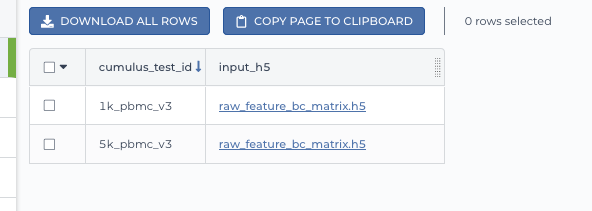
Import cumulus workflow to your workspace as in Case one. Then open
cumulusinWORKFLOWtab. SelectRun workflow(s) with inputs defined by data table, and choose cumulus_test from the drop-down menu.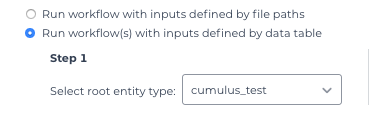
In the input field, specify:
input_file: Typethis.input_h5, wherethisrefers to the data table selected, andinput_h5is the column name in this data table for RNA count matrices.
output_directory: Type Google bucket URL for the main output folder. For example,gs://fc-e0000000-0000-0000-0000-000000000000/cumulus_results.
output_name: Typethis.cumulus_test_id, wherecumulus_test_idis the column name in data table for sample ids.
An example is in the screen shot below:
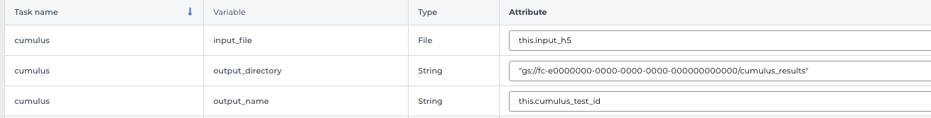
Then finish setting up other inputs following the description in sections below. When you are done, click SAVE, and then RUN ANALYSIS.
When all the jobs are done, you’ll find output for the 2 samples in subfolders gs://fc-e0000000-0000-0000-0000-000000000000/cumulus_results/5k_pbmc_v3 and gs://fc-e0000000-0000-0000-0000-000000000000/cumulus_results/1k_pbmc_v3, respectively.
Cumulus steps:
Cumulus processes single cell data in the following steps:
aggregate_matrices (optional). When given a CSV format sample sheet, this step aggregates channel-specific count matrices into one big count matrix. Users can specify which channels they want to analyze and which sample attributes they want to import to the count matrix in this step. Otherwise, if a single count matrix file is given, skip this step.
cluster. This is the main analysis step. In this step, Cumulus performs low quality cell filtration, highly variable gene selection, batch correction, dimension reduction, diffusion map calculation, graph-based clustering and 2D visualization calculation (e.g. t-SNE/UMAP/FLE).
de_analysis. This step is optional. In this step, Cumulus can calculate potential markers for each cluster by performing a variety of differential expression (DE) analysis. The available DE tests include Welch’s t test, Fisher’s exact test, and Mann-Whitney U test. Cumulus can also calculate the area under ROC (AUROC) curve values for putative markers. If
find_markers_lightgbmis on, Cumulus will try to identify cluster-specific markers by training a LightGBM classifier. If the samples are human or mouse immune cells, Cumulus can also optionally annotate putative cell types for each cluster based on known markers.plot. This step is optional. In this step, Cumulus can generate 6 types of figures based on the cluster step results:
composition plots which are bar plots showing the cell compositions (from different conditions) for each cluster. This type of plots is useful to fast assess library quality and batch effects.
umap and net_umap: UMAP like plots based on different algorithms, respectively. Users can specify cell attributes (e.g. cluster labels, conditions) for coloring side-by-side.
tsne: FIt-SNE plots. Users can specify cell attributes (e.g. cluster labels, conditions) for coloring side-by-side.
fle and net_fle: FLE (Force-directed Layout Embedding) like plots based on different algorithms, respectively. Users can specify cell attributes (e.g. cluster labels, conditions) for coloring side-by-side.
If input is CITE-Seq data, there will be citeseq_umap plots which are UMAP plots based on epitope expression.
cirro_output. This step is optional. Generate Cirrocumulus inputs for visualization using Cirrocumulus .
scp_output. This step is optional. Generate analysis result in Single Cell Portal (SCP) compatible format.
In the following sections, we will first introduce global inputs and then introduce the WDL inputs and outputs for each step separately. But please note that you need to set inputs from all steps simultaneously in the Terra WDL.
Note that we will make the required inputs/outputs bold and all other inputs/outputs are optional.
global inputs
Name |
Description |
Example |
Default |
|---|---|---|---|
input_file |
Input CSV sample sheet describing metadata of each 10x channel, or a single input count matrix file |
“gs://fc-e0000000-0000-0000-0000-000000000000/my_count_matrix.csv” |
|
output_directory |
Google bucket URL of the output directory. |
“gs://fc-e0000000-0000-0000-0000-000000000000/my_results_dir” |
|
output_name |
This is the name of subdirectory for the current sample; and all output files within the subdirectory will have this string as the common filename prefix. |
“my_sample” |
|
default_reference |
If sample count matrix is in either DGE, mtx, csv, tsv or loom format and there is no Reference column in the csv_file, use default_reference as the reference string. |
“GRCh38” |
|
pegasus_version |
Pegasus version to use for analysis. Versions available: |
“1.4.3” |
“1.4.3” |
docker_registry |
Docker registry to use. Options:
|
“quay.io/cumulus” |
“quay.io/cumulus” |
zones |
Google cloud zones to consider for execution. |
“us-east1-d us-west1-a us-west1-b” |
“us-central1-a us-central1-b us-central1-c us-central1-f us-east1-b us-east1-c us-east1-d us-west1-a us-west1-b us-west1-c” |
num_cpu |
Number of CPUs per Cumulus job |
32 |
64 |
memory |
Memory size string |
“200G” |
“200G” |
disk_space |
Total disk space in GB |
100 |
100 |
backend |
Cloud infrastructure backend to use. Available options:
|
“gcp” |
“gcp” |
preemptible |
Number of preemptible tries. This works only when backend is |
2 |
2 |
awsQueueArn |
The AWS ARN string of the job queue to be used. This only works for |
“arn:aws:batch:us-east-1:xxx:job-queue/priority-gwf” |
“” |
aggregate_matrices
aggregate_matrices inputs
Name |
Description |
Example |
Default |
|---|---|---|---|
restrictions |
Select channels that satisfy all restrictions. Each restriction takes the format of name:value,…,value. Multiple restrictions are separated by ‘;’ |
“Source:bone_marrow;Platform:NextSeq” |
|
attributes |
Specify a comma-separated list of outputted attributes. These attributes should be column names in the count_matrix.csv file |
“Source,Platform,Donor” |
|
select_only_singlets |
If we have demultiplexed data, turning on this option will make cumulus only include barcodes that are predicted as singlets. |
true |
false |
remap_singlets |
For demultiplexed data, user can remap singlet names using assignment in String in this input. This string assignment takes the format “new_name_i:old_name_1,old_name_2;new_name_ii:old_name_3;…”.
For example, if we hashed 5 libraries from 3 samples: sample1_lib1, sample1_lib2; sample2_lib1, sample2_lib2; sample3, we can remap them to 3 samples using this string:
"sample1:sample1_lib1,sample1_lib2;sample2:sample2_lib1,sample2_lib2".In this way, the new singlet names will be in metadata field with key
assignment, while the old names are kept in metadata with key assignment.orig.Notice: This input is enabled only when select_only_singlets input is
true. |
“Group1:CB1,CB2;Group2:CB3,CB4,CB5” |
|
subset_singlets |
For demultiplexed data, user can use this input to choose a subset of singlets based on their names. This string takes the format “name1,name2,…”.
Note that if remap_singlets input is specified, subsetting happens after remapping, i.e. you should use the new singlet names for choosing subset.
Notice: This input is enabled only when select_only_singlets input is
true. |
“Group2,CB6,CB7” |
|
minimum_number_of_genes |
Only keep barcodes with at least this number of expressed genes |
100 |
100 |
is_dropseq |
If inputs are DropSeq data. |
false |
false |
aggregate_matrices output
Name |
Type |
Description |
|---|---|---|
output_aggr_zarr |
File |
Aggregated count matrix in Zarr format |
cluster
cluster inputs
Name |
Description |
Example |
Default |
|---|---|---|---|
focus |
Focus analysis on Unimodal data with <keys>. <keys> is a comma-separated list of keys. If None, the
self._selected will be the focused one.Focus key consists of two parts: reference genome name, and data type, connected with a hyphen marker “
-“.Reference genome name depends on the reference you used when running Cellranger workflow. See details in reference list.
|
“GRCh38-rna” |
|
append |
Append Unimodal data <key> to any <keys> in focus.
Similarly as focus keys, append key also consists of two parts: reference genome name, and data type, connected with a hyphen marker “
-“.See reference list for details.
|
“SARSCoV2-rna” |
|
channel |
Specify the cell barcode attribute to represent different samples. |
“Donor” |
|
black_list |
Cell barcode attributes in black list will be poped out. Format is “attr1,attr2,…,attrn”. |
“attr1,attr2,attr3”” |
|
min_genes_before_filtration |
If raw data matrix is input, empty barcodes will dominate pre-filtration statistics. To avoid this, for raw data matrix, only consider barcodes with at least <min_genes_before_filtration> genes for pre-filtration condition. |
100 |
100 |
select_only_singlets |
If we have demultiplexed data, turning on this option will make cumulus only include barcodes that are predicted as singlets |
false |
false |
remap_singlets |
For demultiplexed data, user can remap singlet names using assignment in String in this input. This string assignment takes the format “new_name_i:old_name_1,old_name_2;new_name_ii:old_name_3;…”.
For example, if we hashed 5 libraries from 3 samples: sample1_lib1, sample1_lib2; sample2_lib1, sample2_lib2; sample3, we can remap them to 3 samples using this string:
"sample1:sample1_lib1,sample1_lib2;sample2:sample2_lib1,sample2_lib2".In this way, the new singlet names will be in metadata field with key
assignment, while the old names are kept in metadata with key assignment.orig.Notice: This input is enabled only when select_only_singlets input is
true. |
“Group1:CB1,CB2;Group2:CB3,CB4,CB5” |
|
subset_singlets |
For demultiplexed data, user can use this input to choose a subset of singlets based on their names. This string takes the format “name1,name2,…”.
Note that if remap_singlets is specified, subsetting happens after remapping, i.e. you should use the new singlet names for choosing subset.
Notice: This input is enabled only when select_only_singlets input is
true. |
“Group2,CB6,CB7” |
|
output_filtration_results |
If write cell and gene filtration results to a spreadsheet |
true |
true |
plot_filtration_results |
If plot filtration results as PDF files |
true |
true |
plot_filtration_figsize |
Figure size for filtration plots. <figsize> is a comma-separated list of two numbers, the width and height of the figure (e.g. 6,4) |
6,4 |
|
output_h5ad |
Generate Seurat-compatible h5ad file. Must set to |
true |
true |
output_loom |
If generate loom-formatted file |
false |
false |
min_genes |
Only keep cells with at least <min_genes> of genes |
500 |
500 |
max_genes |
Only keep cells with less than <max_genes> of genes |
6000 |
6000 |
min_umis |
Only keep cells with at least <min_umis> of UMIs. By default, don’t filter cells due to UMI lower bound. |
100 |
|
max_umis |
Only keep cells with less than <max_umis> of UMIs. By default, don’t filter cells due to UMI upper bound. |
600000 |
|
mito_prefix |
Prefix of mitochondrial gene names. This is to identify mitochondrial genes. |
“mt-” |
“MT-” for GRCh38 reference genome data;
“mt-” for mm10 reference genome data;
for other reference genome data, must specify this prefix manually.
|
percent_mito |
Only keep cells with mitochondrial ratio less than <percent_mito>% of total counts |
50 |
20.0 |
gene_percent_cells |
Only use genes that are expressed in at <gene_percent_cells>% of cells to select variable genes |
50 |
0.05 |
counts_per_cell_after |
Total counts per cell after normalization, before transforming the count matrix into Log space. |
1e5 |
1e5 |
select_hvf_flavor |
Highly variable feature selection method. Options:
|
“pegasus” |
“pegasus” |
select_hvf_ngenes |
Select top <select_hvf_ngenes> highly variable features. If <select_hvf_flavor> is “Seurat” and <select_hvf_ngenes> is “None”, select HVGs with z-score cutoff at 0.5. |
2000 |
2000 |
no_select_hvf |
Do not select highly variable features. |
false |
false |
plot_hvf |
Plot highly variable feature selection. Will not work if |
false |
false |
correct_batch_effect |
If correct batch effects |
false |
false |
correction_method |
Batch correction method. Options:
|
“harmony” |
“harmony” |
batch_group_by |
Batch correction assumes the differences in gene expression between channels are due to batch effects.
However, in many cases, we know that channels can be partitioned into several groups and each group is biologically different from others.
In this case, we will only perform batch correction for channels within each group. This option defines the groups.
If <expression> is None, we assume all channels are from one group. Otherwise, groups are defined according to <expression>.
<expression> takes the form of either ‘attr’, or ‘attr1+attr2+…+attrn’, or ‘attr=value11,…,value1n_1;value21,…,value2n_2;…;valuem1,…,valuemn_m’.
In the first form, ‘attr’ should be an existing sample attribute, and groups are defined by ‘attr’.
In the second form, ‘attr1’,…,’attrn’ are n existing sample attributes and groups are defined by the Cartesian product of these n attributes.
In the last form, there will be m + 1 groups.
A cell belongs to group i (i > 0) if and only if its sample attribute ‘attr’ has a value among valuei1,…,valuein_i.
A cell belongs to group 0 if it does not belong to any other groups
|
“Donor” |
None |
random_state |
Random number generator seed |
0 |
0 |
calc_signature_scores |
Gene set for calculating signature scores. It can be either of the following forms:
|
“cell_cycle_human” |
|
nPC |
Number of principal components |
50 |
50 |
knn_K |
Number of nearest neighbors used for constructing affinity matrix. |
50 |
100 |
knn_full_speed |
For the sake of reproducibility, we only run one thread for building kNN indices. Turn on this option will allow multiple threads to be used for index building. However, it will also reduce reproducibility due to the racing between multiple threads. |
false |
false |
run_diffmap |
Whether to calculate diffusion map or not. It will be automatically set to |
false |
false |
diffmap_ndc |
Number of diffusion components |
100 |
100 |
diffmap_maxt |
Maximum time stamp in diffusion map computation to search for the knee point. |
5000 |
5000 |
run_louvain |
Run Louvain clustering algorithm |
true |
true |
louvain_resolution |
Resolution parameter for the Louvain clustering algorithm |
1.3 |
1.3 |
louvain_class_label |
Louvain cluster label name in analysis result. |
“louvain_labels” |
“louvain_labels” |
run_leiden |
Run Leiden clustering algorithm. |
false |
false |
leiden_resolution |
Resolution parameter for the Leiden clustering algorithm. |
1.3 |
1.3 |
leiden_niter |
Number of iterations of running the Leiden algorithm. If negative, run Leiden iteratively until no improvement. |
2 |
-1 |
leiden_class_label |
Leiden cluster label name in analysis result. |
“leiden_labels” |
“leiden_labels” |
run_spectral_louvain |
Run Spectral Louvain clustering algorithm |
false |
false |
spectral_louvain_basis |
Basis used for KMeans clustering. Use diffusion map by default. If diffusion map is not calculated, use PCA coordinates. Users can also specify “pca” to directly use PCA coordinates. |
“diffmap” |
“diffmap” |
spectral_louvain_resolution |
Resolution parameter for louvain. |
1.3 |
1.3 |
spectral_louvain_class_label |
Spectral louvain label name in analysis result. |
“spectral_louvain_labels” |
“spectral_louvain_labels” |
run_spectral_leiden |
Run Spectral Leiden clustering algorithm. |
false |
false |
spectral_leiden_basis |
Basis used for KMeans clustering. Use diffusion map by default. If diffusion map is not calculated, use PCA coordinates. Users can also specify “pca” to directly use PCA coordinates. |
“diffmap” |
“diffmap” |
spectral_leiden_resolution |
Resolution parameter for leiden. |
1.3 |
1.3 |
spectral_leiden_class_label |
Spectral leiden label name in analysis result. |
“spectral_leiden_labels” |
“spectral_leiden_labels” |
run_tsne |
Run FIt-SNE for visualization. |
false |
false |
tsne_perplexity |
t-SNE’s perplexity parameter. |
30 |
30 |
tsne_initialization |
Initialization method for FIt-SNE. It can be either: ‘random’ refers to random initialization; ‘pca’ refers to PCA initialization as described in [Kobak et al. 2019]. |
“pca” |
“pca” |
run_umap |
Run UMAP for visualization |
true |
true |
umap_K |
K neighbors for UMAP. |
15 |
15 |
umap_min_dist |
UMAP parameter. |
0.5 |
0.5 |
umap_spread |
UMAP parameter. |
1.0 |
1.0 |
run_fle |
Run force-directed layout embedding (FLE) for visualization |
false |
false |
fle_K |
Number of neighbors for building graph for FLE |
50 |
50 |
fle_target_change_per_node |
Target change per node to stop FLE. |
2.0 |
2.0 |
fle_target_steps |
Maximum number of iterations before stopping the algoritm |
5000 |
5000 |
net_down_sample_fraction |
Down sampling fraction for net-related visualization |
0.1 |
0.1 |
run_net_umap |
Run Net UMAP for visualization |
false |
false |
net_umap_out_basis |
Basis name for Net UMAP coordinates in analysis result |
“net_umap” |
“net_umap” |
run_net_fle |
Run Net FLE for visualization |
false |
false |
net_fle_out_basis |
Basis name for Net FLE coordinates in analysis result. |
“net_fle” |
“net_fle” |
infer_doublets |
Infer doublets using the Pegasus method. When finished, Scrublet-like doublet scores are in cell attribute |
false |
false |
expected_doublet_rate |
The expected doublet rate per sample. If not specified, calculate the expected rate based on number of cells from the 10x multiplet rate table. |
0.05 |
|
doublet_cluster_attribute |
Specify which cluster attribute (e.g. “louvain_labels”) should be used for doublet inference. Then doublet clusters will be marked with the following criteria: passing the Fisher’s exact test and having >= 50% of cells identified as doublets.
If not specified, the first computed cluster attribute in the list of “leiden”, “louvain”, “spectral_ledein” and “spectral_louvain” will be used.
|
“louvain_labels” |
|
citeseq |
Perform CITE-Seq data analysis. Set to
true if input data contain both RNA and CITE-Seq modalities.This will set focus to be the RNA modality and append to be the CITE-Seq modality. In addition,
"ADT-" will be added in front of each antibody name to avoid name conflict with genes in the RNA modality. |
false |
false |
citeseq_umap |
For high quality cells kept in the RNA modality, calculate a distinct UMAP embedding based on their antibody expression. |
false |
false |
citeseq_umap_exclude |
A comma-separated list of antibodies to be excluded from the CITE-Seq UMAP calculation (e.g. Mouse-IgG1,Mouse-IgG2a). |
“Mouse-IgG1,Mouse-IgG2a” |
cluster outputs
Name |
Type |
Description |
|---|---|---|
output_zarr |
File |
Output file in zarr format (output_name.zarr.zip).
To load this file in Python, you need to first install PegasusIO on your local machine. Then use
import pegasusio as io; data = io.read_input('output_name.zarr.zip') in Python environment.data is a MultimodalData object, and points to its default UnimodalData element. You can set its default UnimodalData to others by data.set_data(focus_key) where focus_key is the key string to the wanted UnimodalData element.For its default UnimodalData element, the log-normalized expression matrix is stored in
data.X as a Scipy CSR-format sparse matrix, with cell-by-gene shape.Alternatively, to get the raw count matrix, first run
data.select_matrix('raw.X'), then data.X will be switched to point to the raw matrix.The
obs field contains cell related attributes, including clustering results.For example,
data.obs_names records cell barcodes; data.obs['Channel'] records the channel each cell comes from;data.obs['n_genes'], data.obs['n_counts'], and data.obs['percent_mito'] record the number of expressed genes, total UMI count, and mitochondrial rate for each cell respectively;data.obs['louvain_labels'], data.obs['leiden_labels'], data.obs['spectral_louvain_labels'], and data.obs['spectral_leiden_labels'] record each cell’s cluster labels using different clustering algorithms;The
var field contains gene related attributes.For example,
data.var_names records gene symbols, data.var['gene_ids'] records Ensembl gene IDs, and data.var['highly_variable_features'] records selected variable genes.The
obsm field records embedding coordinates.For example,
data.obsm['X_pca'] records PCA coordinates, data.obsm['X_tsne'] records t-SNE coordinates,data.obsm['X_umap'] records UMAP coordinates, data.obsm['X_diffmap'] records diffusion map coordinates,and
data.obsm['X_fle'] records the force-directed layout coordinates.The
uns field stores other related information, such as reference genome (data.uns['genome']), kNN on PCA coordinates (data.uns['pca_knn_indices'] and data.uns['pca_knn_distances']), etc. |
output_log |
File |
This is a copy of the logging module output, containing important intermediate messages |
output_h5ad |
Array[File] |
List of output file(s) in Seurat-compatible h5ad format (output_name.focus_key.h5ad), in which each file is associated with a focus of the input data.
To load this file in Python, first install PegasusIO on your local machine. Then use
import pegasusio as io; data = io.read_input('output_name.focus_key.h5ad') in Python environment.After loading,
data has the similar structure as UnimodalData object in Description of output_zarr in cluster outputs section.In addition,
data.uns['scale.data'] records variable-gene-selected and standardized expression matrix which are ready to perform PCA, and data.uns['scale.data.rownames'] records indexes of the selected highly variable genes.This file is used for loading in R and converting into a Seurat object (see here for instructions)
|
output_filt_xlsx |
File |
Spreadsheet containing filtration results (output_name.filt.xlsx).
This file has two sheets — Cell filtration stats and Gene filtration stats.
The first sheet records cell filtering results and it has 10 columns:
Channel, channel name; kept, number of cells kept; median_n_genes, median number of expressed genes in kept cells; median_n_umis, median number of UMIs in kept cells;
median_percent_mito, median mitochondrial rate as UMIs between mitochondrial genes and all genes in kept cells;
filt, number of cells filtered out; total, total number of cells before filtration, if the input contain all barcodes, this number is the cells left after ‘min_genes_on_raw’ filtration;
median_n_genes_before, median expressed genes per cell before filtration; median_n_umis_before, median UMIs per cell before filtration;
median_percent_mito_before, median mitochondrial rate per cell before filtration.
The channels are sorted in ascending order with respect to the number of kept cells per channel.
The second sheet records genes that failed to pass the filtering.
This sheet has 3 columns: gene, gene name; n_cells, number of cells this gene is expressed; percent_cells, the fraction of cells this gene is expressed.
Genes are ranked in ascending order according to number of cells the gene is expressed.
Note that only genes not expressed in any cell are removed from the data.
Other filtered genes are marked as non-robust and not used for TPM-like normalization
|
output_filt_plot |
Array[File] |
If not empty, this array contains 3 PDF files.
output_name.filt.gene.pdf, which contains violin plots contrasting gene count distributions before and after filtration per channel.
output_name.filt.UMI.pdf, which contains violin plots contrasting UMI count distributions before and after filtration per channel.
output_name.filt.mito.pdf, which contains violin plots contrasting mitochondrial rate distributions before and after filtration per channel
|
output_hvf_plot |
Array[File] |
If not empty, this array contains PDF files showing scatter plots of genes upon highly variable feature selection. |
output_dbl_plot |
Array[File] |
If infer_doublets input field is |
output_loom_file |
Array[File] |
List of output file in loom format (output_name.focus_key.loom), in which each file is associated with a focus of the input data.
To load this file in Python, first install loompy. Then type
from loompy import connect; ds = connect('output_name.focus_key.loom') in Python environment.The log-normalized expression matrix is stored in
ds with gene-by-cell shape. ds[:, :] returns the matrix in dense format; ds.layers[''].sparse() returns it as a Scipy COOrdinate sparse matrix.The
ca field contains cell related attributes as row attributes, including clustering results and cell embedding coordinates.For example,
ds.ca['obs_names'] records cell barcodes; ds.ca['Channel'] records the channel each cell comes from;ds.ca['louvain_labels'], ds.ca['leiden_labels'], ds.ca['spectral_louvain_labels'], and ds.ca['spectral_leiden_labels'] record each cell’s cluster labels using different clustering algorithms;ds.ca['X_pca'] records PCA coordinates, ds.ca['X_tsne'] records t-SNE coordinates,ds.ca['X_umap'] records UMAP coordinates, ds.ca['X_diffmap'] records diffusion map coordinates,and
ds.ca['X_fle'] records the force-directed layout coordinates.The
ra field contains gene related attributes as column attributes.For example,
ds.ra['var_names'] records gene symbols, ds.ra['gene_ids'] records Ensembl gene IDs, and ds.ra['highly_variable_features'] records selected variable genes. |
de_analysis
de_analysis inputs
Name |
Description |
Example |
Default |
|---|---|---|---|
perform_de_analysis |
Whether perform differential expression (DE) analysis. If performing, by default calculate AUROC scores and Mann-Whitney U test. |
true |
true |
cluster_labels |
Specify the cluster label used for DE analysis |
“louvain_labels” |
“louvain_labels” |
alpha |
Control false discovery rate at <alpha> |
0.05 |
0.05 |
fisher |
Calculate Fisher’s exact test |
false |
false |
t_test |
Calculate Welch’s t-test. |
false |
false |
find_markers_lightgbm |
If also detect markers using LightGBM |
false |
false |
remove_ribo |
Remove ribosomal genes with either RPL or RPS as prefixes. Currently only works for human data |
false |
false |
min_gain |
Only report genes with a feature importance score (in gain) of at least <gain> |
1.0 |
1.0 |
annotate_cluster |
If also annotate cell types for clusters based on DE results |
false |
false |
annotate_de_test |
Differential Expression test to use for inference on cell types. Options: |
“mwu” |
“mwu” |
organism |
Organism, could either of the follow:
|
“mouse_immune,mouse_brain” |
“human_immune” |
minimum_report_score |
Minimum cell type score to report a potential cell type |
0.5 |
0.5 |
de_analysis outputs
Name |
Type |
Description |
|---|---|---|
output_de_h5ad |
Array[File] |
List of h5ad-formatted results with DE results updated (output_name.focus_key.h5ad), in which each file is associated with a focus of the input data.
To load this file in Python, you need to first install PegasusIO on your local machine. Then type
import pegasusio as io; data = io.read_input('output_name.focus_key.h5ad') in Python environment.After loading,
data has the similar structure as UnimodalData object in Description of output_zarr in cluster outputs section.Besides, there is one additional field
varm which records DE analysis results in data.varm['de_res']. You can use Pandas DataFrame to convert it into a reader-friendly structure: import pandas as pd; df = pd.DataFrame(data.varm['de_res'], index=data.var_names). Then in the resulting data frame, genes are rows, and those DE test statistics are columns.DE analysis in cumulus is performed on each cluster against cells in all the other clusters. For instance, in the data frame, column
1:log2Mean refers to the mean expression of genes in log-scale for cells in Cluster 1. The number before colon refers to the cluster label to which this statistic belongs. |
output_de_xlsx |
Array[File] |
List of spreadsheets reporting DE results (output_name.focus_key.de.xlsx), in which each file is associated with a focus of the input data.
Each cluster has two tabs: one for up-regulated genes for this cluster, one for down-regulated ones. In each tab, genes are ranked by AUROC scores.
Genes which are not significant in terms of q-values in any of the DE test are not included (at false discovery rate specified in alpha field of de_analysis inputs).
|
output_markers_xlsx |
Array[File] |
List of Excel spreadsheets containing detected markers (output_name.focus_key.markers.xlsx), in which each file is associated with a focus of the input data. Each cluster has one tab in the spreadsheet and each tab has three columns, listing markers that are strongly up-regulated, weakly up-regulated and down-regulated. |
output_anno_file |
Array[File] |
List of cluster-based cell type annotation files (output_name.focus_key.anno.txt), in which each file is associated with a focus of the input data. |
How cell type annotation works
In this subsection, we will describe the format of input JSON cell type marker file, the ad hoc cell type inference algorithm, and the format of the output putative cell type file.
JSON file
The top level of the JSON file is an object with two name/value pairs:
title: A string to describe what this JSON file is for (e.g. “Mouse brain cell markers”).
cell_types: List of all cell types this JSON file defines. In this list, each cell type is described using a separate object with 2 to 3 name/value pairs:
name: Cell type name (e.g. “GABAergic neuron”).
markers: List of gene-marker describing objects, each of which has 2 name/value pairs:
genes: List of positive and negative gene markers (e.g.
["Rbfox3+", "Flt1-"]).weight: A real number between
0.0and1.0to describe how much we trust the markers in genes.All markers in genes share the weight evenly. For instance, if we have 4 markers and the weight is 0.1, each marker has a weight of
0.1 / 4 = 0.025.The weights from all gene-marker describing objects of the same cell type should sum up to 1.0.
subtypes: Description on cell subtypes for the cell type. It has the same structure as the top level JSON object.
See below for an example JSON snippet:
{
  "title" : "Mouse brain cell markers",
    "cell_types" : [
      {
        "name" : "Glutamatergic neuron",
        "markers" : [
          {
            "genes" : ["Rbfox3+", "Reln+", "Slc17a6+", "Slc17a7+"],
            "weight" : 1.0
          }
        ],
        "subtypes" : {
          "title" : "Glutamatergic neuron subtype markers",
            "cell_types" : [
              {
                "name" : "Glutamatergic layer 4",
                "markers" : [
                  {
                    "genes" : ["Rorb+", "Paqr8+"],
                    "weight" : 1.0
                  }
                ]
              }
            ]
        }
      }
    ]
}
Inference Algorithm
We have already calculated the up-regulated and down-regulated genes for each cluster in the differential expression analysis step.
First, load gene markers for each cell type from the JSON file specified, and exclude marker genes, along with their associated weights, that are not expressed in the data.
Then scan each cluster to determine its putative cell types. For each cluster and putative cell type, we calculate a score between 0 and 1, which describes how likely cells from the cluster are of this cell type. The higher the score is, the more likely cells are from the cell type.
To calculate the score, each marker is initialized with a maximum impact value (which is 2). Then do case analysis as follows:
For a positive marker:
If it is not up-regulated, its impact value is set to
0.Otherwise, if it is up-regulated:
If it additionally has a fold change in percentage of cells expressing this marker (within cluster vs. out of cluster) no less than
1.5, it has an impact value of2and is recorded as a strong supporting marker.If its fold change (
fc) is less than1.5, this marker has an impact value of1 + (fc - 1) / 0.5and is recorded as a weak supporting marker.For a negative marker:
If it is up-regulated, its impact value is set to
0.If it is neither up-regulated nor down-regulated, its impact value is set to
1.Otherwise, if it is down-regulated:
If it additionally has
1 / fc(wherefcis its fold change) no less than1.5, it has an impact value of2and is recorded as a strong supporting marker.If
1 / fcis less than1.5, it has an impact value of1 + (1 / fc - 1) / 0.5and is recorded as a weak supporting marker.
The score is calculated as the weighted sum of impact values weighted over the sum of weights multiplied by 2 from all expressed markers. If the score is larger than 0.5 and the cell type has cell subtypes, each cell subtype will also be evaluated.
Output annotation file
For each cluster, putative cell types with scores larger than minimum_report_score will be reported in descending order with respect to their scores. The report of each putative cell type contains the following fields:
name: Cell type name.
score: Score of cell type.
average marker percentage: Average percentage of cells expressing marker within the cluster between all positive supporting markers.
strong support: List of strong supporting markers. Each marker is represented by a tuple of its name and percentage of cells expressing it within the cluster.
weak support: List of week supporting markers. It has the same structure as strong support.
plot
The h5ad file contains a default cell attribute Channel, which records which channel each that single cell comes from. If the input is a CSV format sample sheet, Channel attribute matches the Sample column in the sample sheet. Otherwise, it’s specified in channel field of the cluster inputs.
Other cell attributes used in plot must be added via attributes field in the aggregate_matrices inputs.
plot inputs
Name |
Description |
Example |
Default |
|---|---|---|---|
plot_composition |
Takes the format of “label:attr,label:attr,…,label:attr”.
If non-empty, generate composition plot for each “label:attr” pair.
“label” refers to cluster labels and “attr” refers to sample conditions
|
“louvain_labels:Donor” |
None |
plot_tsne |
Takes the format of “attr,attr,…,attr”.
If non-empty, plot attr colored FIt-SNEs side by side
|
“louvain_labels,Donor” |
None |
plot_umap |
Takes the format of “attr,attr,…,attr”.
If non-empty, plot attr colored UMAP side by side
|
“louvain_labels,Donor” |
None |
plot_fle |
Takes the format of “attr,attr,…,attr”.
If non-empty, plot attr colored FLE (force-directed layout embedding) side by side
|
“louvain_labels,Donor” |
None |
plot_net_umap |
Takes the format of “attr,attr,…,attr”.
If non-empty, plot attr colored UMAP side by side based on net UMAP result.
|
“leiden_labels,Donor” |
None |
plot_net_fle |
Takes the format of “attr,attr,…,attr”.
If non-empty, plot attr colored FLE (force-directed layout embedding) side by side
based on net FLE result.
|
“leiden_labels,Donor” |
None |
plot_citeseq_umap |
Takes the format of “attr,attr,…,attr”.
If non-empty, plot attr colored UMAP side by side based on CITE-Seq UMAP result.
|
“louvain_labels,Donor” |
None |
plot outputs
Name |
Type |
Description |
|---|---|---|
output_pdfs |
Array[File] |
Outputted pdf files |
output_htmls |
Array[File] |
Outputted html files |
Generate input files for Cirrocumulus
Generate Cirrocumulus inputs for visualization using Cirrocumulus .
cirro_output inputs
Name |
Description |
Example |
Default |
|---|---|---|---|
generate_cirro_inputs |
Whether to generate input files for Cirrocumulus |
false |
false |
cirro_output outputs
Name |
Type |
Description |
|---|---|---|
output_cirro_path |
Google Bucket URL |
Path to Cirrocumulus inputs |
Generate SCP-compatible output files
Generate analysis result in Single Cell Portal (SCP) compatible format.
scp_output inputs
Name |
Description |
Example |
Default |
|---|---|---|---|
generate_scp_outputs |
Whether to generate SCP format output or not. |
false |
false |
output_dense |
Output dense expression matrix, instead of the default sparse matrix format. |
false |
false |
scp_output outputs
Name |
Type |
Description |
|---|---|---|
output_scp_files |
Array[File] |
Outputted SCP format files. |
Run CITE-Seq analysis
Users now can use cumulus/cumulus workflow solely to run CITE-Seq analysis.
Prepare a sample sheet in the following format:
Sample,Location,Modality
sample_1,gs://your-bucket/rna_raw_counts.h5,rna
sample_1,gs://your-bucket/citeseq_cell_barcodes.csv,citeseq
Each row stands for one modality:
Sample: Sample name, which must be the same in the two rows to let Cumulus aggregate RNA and CITE-Seq matrices.
Location: Google bucket URL of the corresponding count matrix file.
Modality: Modality type.
rnafor RNA count matrix;citeseqfor CITE-Seq antibody count matrix.
Run cumulus/cumulus workflow using this sample sheet as the input file, and specify the following input fields:
citeseq: Set this to
trueto enable CITE-Seq analysis.citeseq_umap: Set this to
trueto calculate the CITE-Seq UMAP embedding on cells.citeseq_umap_exclude: A list of CITE-Seq antibodies to be excluded from UMAP calculation. This list should be written in a string format with each antobidy name separated by comma.
plot_citeseq_umap: A list of cell barcode attributes to be plotted based on CITE-Seq UMAP embedding. This list should be written in a string format with each attribute separated by comma.
Load Cumulus results into Pegasus
Pegasus is a Python package for large-scale single-cell/single-nucleus data analysis, and it uses PegasusIO for read/write. To load Cumulus results into Pegasus, we provide instructions based on file format:
zarr: Annotated Zarr file in zip format. This is the standard output format of Cumulus. You can load it by:
import pegasusio as io
data = io.read_input("output_name.zarr.zip")
h5ad: When setting “output_h5ad” field in Cumulus cluster to true, a list of annotated H5AD file(s) will be generated besides Zarr result. If the input data have multiple foci, Cumulus will generate one H5AD file per focus. You can load it by:
import pegasusio as io
adata = io.read_input("output_name.focus_key.h5ad")
Sometimes you may also want to specify how the result is loaded into memory. In this case, read_input has argument mode. Please see its documentation for details.
loom: When setting “output_loom” field in Cumulus cluster to true, a list of loom format file(s) will be generated besides Zarr result. Similarly as H5AD output, Cumulus generates multiple loom files if the input data have more than one foci. To load loom file, you can optionally set its genome name in the following way as this information is not contained by loom file:
import pegasusio as io
data = pg.read_input("output_name.focus_key.loom", genome = "GRCh38")
After loading, Pegasus manipulate the data matrix in PegasusIO MultimodalData structure.
Load Cumulus results into Seurat
Seurat is a single-cell data analysis package written in R.
Load H5AD File into Seurat
First, you need to set “output_h5ad” field to true in cumulus cluster inputs to generate Seurat-compatible output files output_name.focus_key.h5ad, in addition to the standard result output_name.zarr.zip. If the input data have multiple foci, Cumulus will generate one H5AD file per focus.
Notice that Python, and Python package anndata with version at least 0.6.22.post1, and R package reticulate are required to load the result into Seurat.
Execute the R code below to load the h5ad result into Seurat (working with both Seurat v2 and v3):
source("https://raw.githubusercontent.com/lilab-bcb/cumulus/master/workflows/cumulus/h5ad2seurat.R")
ad <- import("anndata", convert = FALSE)
test_ad <- ad$read_h5ad("output_name.focus_key.h5ad")
result <- convert_h5ad_to_seurat(test_ad)
The resulting Seurat object result has three data slots:
raw.data records filtered raw count matrix.
data records filtered and log-normalized expression matrix.
scale.data records variable-gene-selected, standardized expression matrix that are ready to perform PCA.
Load loom File into Seurat
First, you need to set “output_loom” field to true in cumulus cluster inputs to generate a loom format output file, say output_name.focus_key.loom, in addition to the standard result output_name.zarr.zip. If the input data have multiple foci, Cumulus will generate one loom file per focus.
You also need to install loomR package in your R environment:
install.package("devtools")
devtools::install_github("mojaveazure/loomR", ref = "develop")
Execute the R code below to load the loom file result into Seurat (working with Seurat v3 only):
source("https://raw.githubusercontent.com/lilab-bcb/cumulus/master/workflows/cumulus/loom2seurat.R")
result <- convert_loom_to_seurat("output_name.focus_key.loom")
In addition, if you want to set an active cluster label field for the resulting Seurat object, do the following:
Idents(result) <- result@meta.data$louvain_labels
where louvain_labels is the key to the Louvain clustering result in Cumulus, which is stored in cell attributes result@meta.data.
Load Cumulus results into SCANPY
SCANPY is another Python package for single-cell data analysis. We provide instructions on loading Cumulus output into SCANPY based on file format:
h5ad: Annotated H5AD file. This is the standard output format of Cumulus:
import scanpy as sc
adata = sc.read_h5ad("output_name.h5ad")
Sometimes you may also want to specify how the result is loaded into memory. In this case, read_h5ad has argument backed. Please see SCANPY documentation for details.
loom: This format is generated when setting “output_loom” field in Cumulus cluster to true:
import scanpy as sc
adata = sc.read_loom("output_name.loom")
Besides, read_loom has a boolean sparse argument to decide whether to read the data matrix as sparse, with default value True. If you want to load it as a dense matrix, simply type:
adata = sc.read_loom("output_name.loom", sparse = False)
After loading, SCANPY manipulates the data matrix in anndata structure.
Visualize Cumulus results in Python
Ensure you have Pegasus installed.
Download your analysis result data, say output_name.zarr.zip, from Google bucket to your local machine.
Follow Pegasus plotting tutorial for visualizing your data in Python.